ROS 2 Demonstration-Based Trajectory Tracking for a 2-DOF Planar Robot
ROS 2 Python project for demonstration-trajectory replay, joint-space PD control, simulated 2-DOF planar robot dynamics, disturbance injection, and quantitative tracking-error analysis.
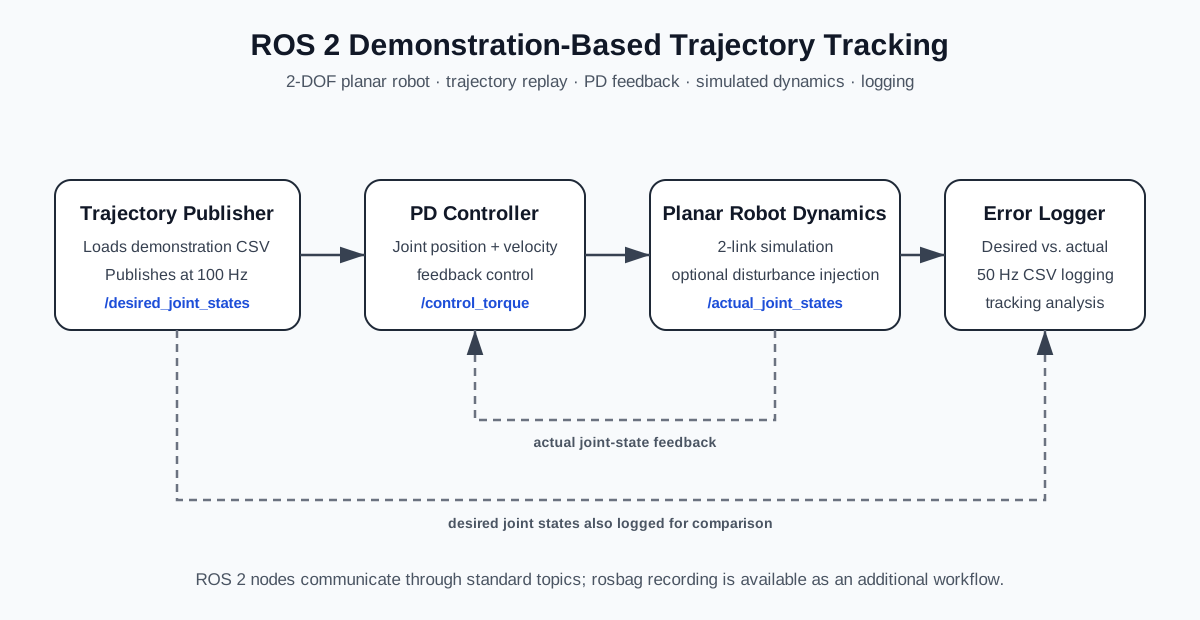
This ROS 2 project implements a compact closed-loop software pipeline for replaying a joint-space demonstration trajectory and tracking it on a simulated two-degree-of-freedom planar robot. I separated the reference publisher, feedback controller, dynamics simulator, and tracking logger into independent ROS 2 nodes so that the communication, control, disturbance, and analysis workflow can be inspected and extended clearly.
The project is available here: GitHub repository
The current version was built and run with ROS 2 Jazzy. A disturbed simulation using the current public controller tuning produced 3,554 logged samples over 71.08 seconds. The quantitative results below are computed from that recorded CSV file and include the initial convergence transient.
ROS 2 control architecture
The demonstration trajectory is loaded from config/demo_trajectory.csv and published on /desired_joint_states. The controller combines this reference with feedback from /actual_joint_states and publishes the two-joint command on /control_torque. The simulation and controller both operate at 100 Hz, while the tracking logger records the desired and actual states at 50 Hz.
| ROS 2 component | Interface / rate |
|---|---|
| Trajectory publisher | /desired_joint_states · 100 Hz |
| PD controller | /control_torque · 100 Hz |
| Planar dynamics | /actual_joint_states · 100 Hz |
| Tracking logger | CSV output · 50 Hz |
Feedback controller and simulated dynamics
The controller is intentionally simple: joint-position and joint-velocity errors are mapped to torque commands using a saturated PD law. The current public launch configuration uses Kp = [30, 12], Kd = [5, 1.5], and a torque limit of ±20 N·m in the simulated model.
tau = Kp * (q_des - q) + Kd * (qdot_des - qdot)The plant is a lightweight horizontal two-link rigid-body model with viscous friction. Its simulated dynamics are evaluated numerically at 100 Hz and include optional additive joint disturbances.
M(q) qddot + C(q, qdot) + B qdot = tau + disturbance| Simulation setting | Value |
|---|---|
| Proportional gains | [30, 12] |
| Derivative gains | [5, 1.5] |
| Torque saturation | ±20 N·m |
| Stochastic disturbance standard deviation | 0.15 N·m |
| Sinusoidal disturbance amplitude | 0.25 N·m |
The disturbance parameters belong to the simulated joint-torque model. They are not measurements of noise or external loading from a physical robot.
Measured trajectory tracking
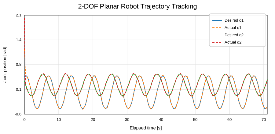
The final recorded dataset contains 3,554 samples spanning 71.08 seconds. Tracking metrics are calculated directly from the logged joint-position errors over the complete recording, including the startup transient.
| Tracking metric | Measured value |
|---|---|
| Joint 1 RMSE | 0.03397 rad |
| Joint 2 RMSE | 0.06120 rad |
| Mean joint-error norm | 0.01873 rad |
| Logged samples | 3,554 |
| Recorded duration | 71.08 s |
These numbers describe this specific simulation run. They should not be interpreted as physical robot accuracy, a statistical robustness guarantee, or performance across untested robot models and disturbance conditions.
Tracking error under disturbance
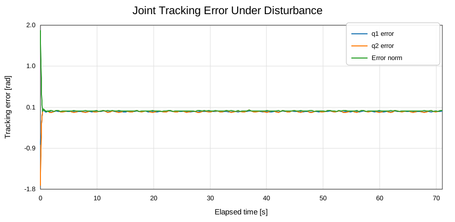
The error norm is computed from the two joint-position errors at each logged sample. The relatively large initial transient is retained rather than removed from the reported RMSE values, so the quantitative summary reflects the complete saved run rather than only a selected steady portion.
Relation to learning-based robot control
This project does not implement reinforcement learning. Its role is to provide a small and readable ROS 2 control baseline that already contains the interfaces needed for later learning-based experiments: desired-state publishing, state feedback, torque commands, disturbance injection, synchronized logging, and quantitative analysis. A future residual-learning controller could therefore be added without changing the basic data flow of the package.
Scope and limitations
The current project is software- and simulation-based. The robot is represented by a simplified 2-DOF planar rigid-body model, the demonstration is a predefined CSV trajectory rather than motion recorded from a human or physical robot, and the feedback controller is PD rather than a learned policy. The project does not use Gazebo, MuJoCo, PyBullet, or a physical robotic platform.
The reported metrics come from one disturbed simulation run with the documented controller and disturbance settings. No Monte Carlo robustness study, formal stability proof, hardware experiment, or cross-distribution ROS 2 validation is claimed. The current workflow has been executed successfully with ROS 2 Jazzy.
Reproducibility
The repository contains the ROS 2 Python package, launch file, demonstration CSV, plotting scripts, rosbag helper, and tracking logger. A clean Jazzy workspace can build and launch the complete pipeline with the commands below.
mkdir -p ~/ros2_ws/src
cd ~/ros2_ws/src
git clone https://github.com/mhfakouri/ros2-planar-robot-trajectory-tracking.git

cd ~/ros2_ws
source /opt/ros/jazzy/setup.bash
colcon build --symlink-install
source install/setup.bash

ros2 launch ros2_demo_based_tracking demo_tracking.launch.py
By default, the logger writes to /tmp/ros2_demo_tracking_log.csv. The repository's plotting script reads that CSV and computes the RMSE and mean error-norm values used in the results summary.