Polynomial Robot Motion Planning
MATLAB project comparing cubic, quintic, and corrected LSPB joint-space trajectories with boundary-condition verification, trajectory derivatives, and explicit correction of archived formulation errors.
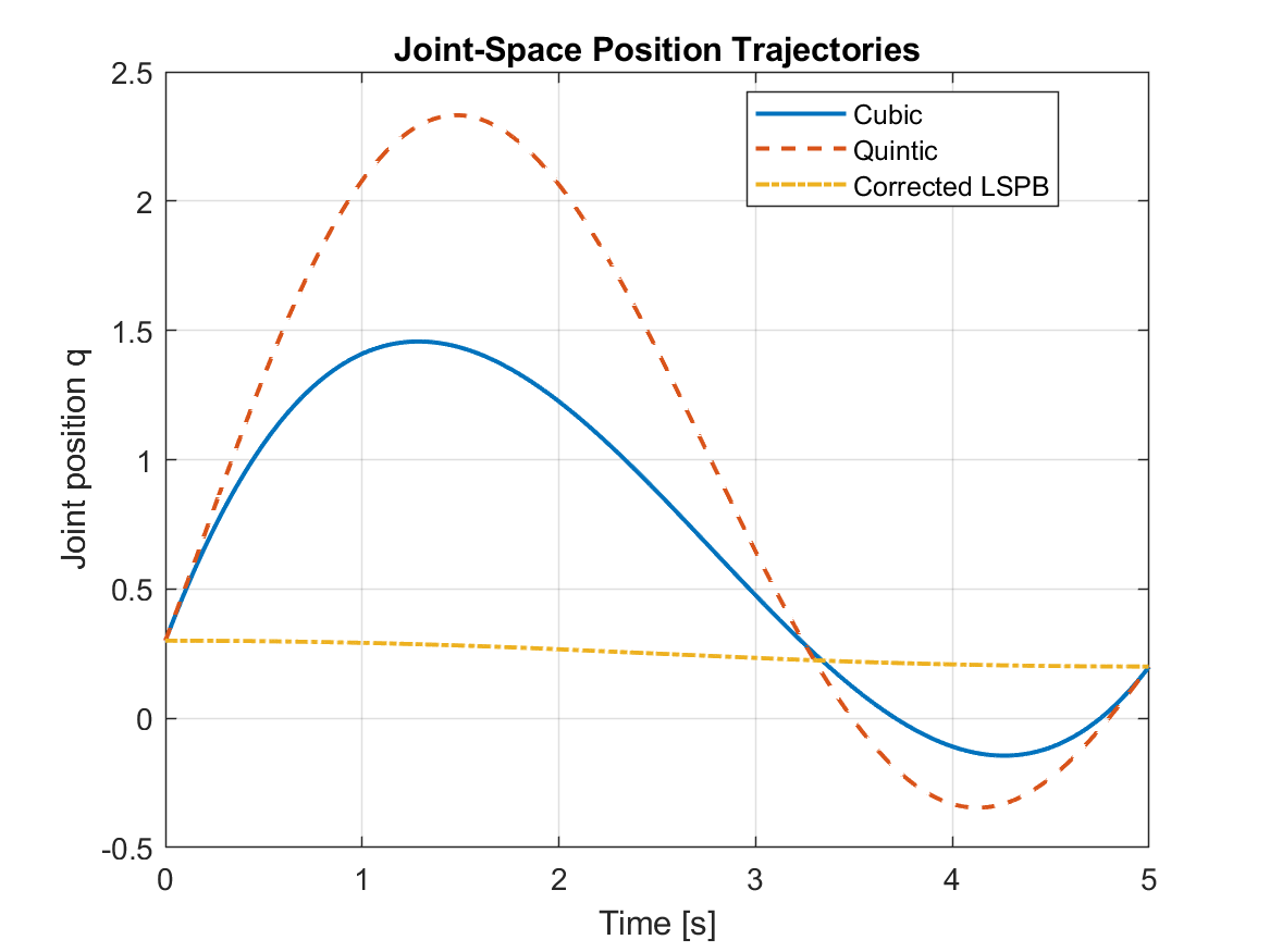
This MATLAB project compares three classical joint-space trajectory-generation methods: a cubic polynomial, a quintic polynomial, and a linear-segment-with-parabolic-blends (LSPB) construction. I reorganized the archived coursework into one reproducible workflow that verifies endpoint conditions numerically, compares trajectory derivatives, and explicitly documents two source inconsistencies that had to be corrected before publication.
The complete implementation and generated results are available here: GitHub repository
The cleaned version keeps the original boundary-value problem and trajectory families, but it does not silently repeat the flawed archived formulas. Instead, it validates each construction directly and separates what the cubic, quintic, and corrected LSPB trajectories can actually satisfy.
Source-derived boundary-value problem
The archived motion-planning task defines a single generalized coordinate q(t) with the following endpoint conditions:
| Boundary condition | Value |
|---|---|
q(0) | 0.3 |
q̇(0) | 2.0 |
q̈(0) | 1.0 |
q(tf) | 0.2 |
q̇(tf) | 1.0 |
q̈(tf) | 0.0 |
tf | 5.0 s |
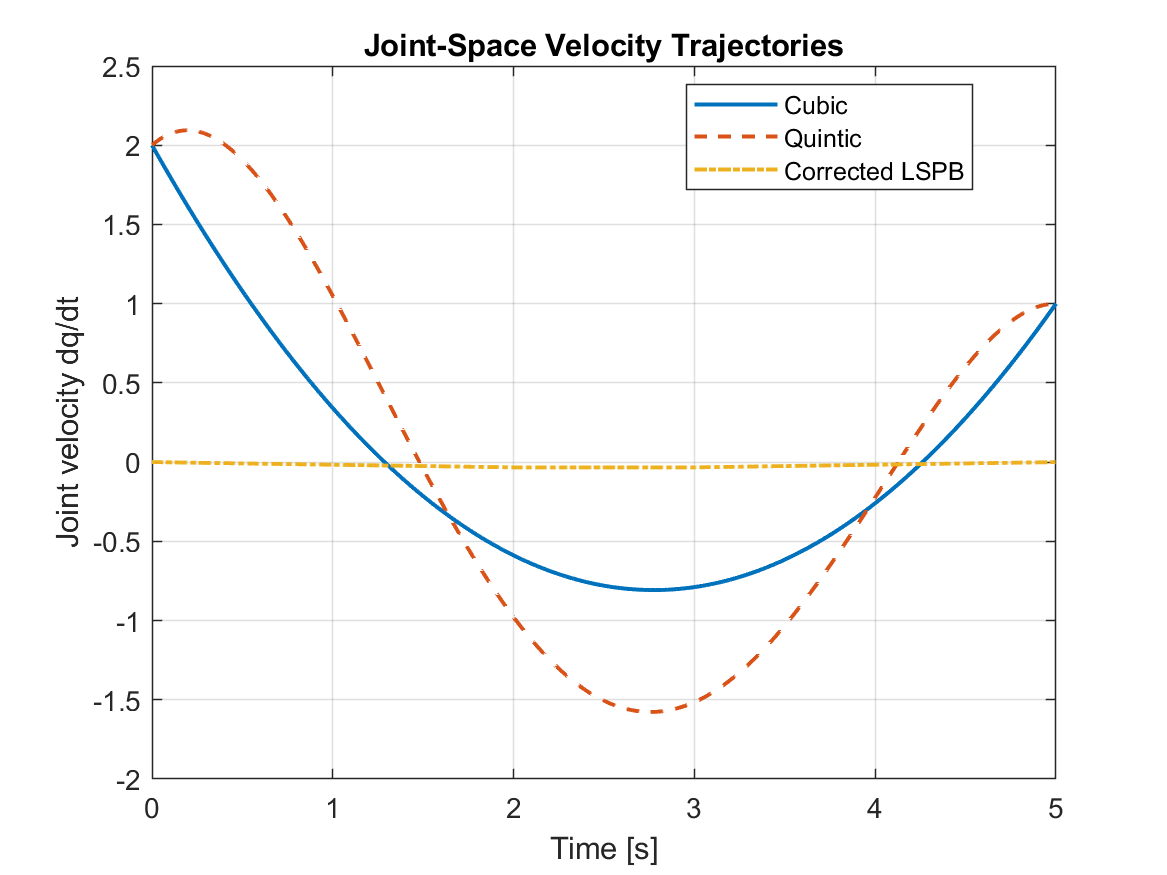
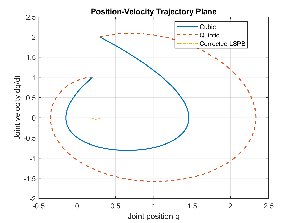
One subtle feature of this problem is that the net displacement is negative (qf − q0 = −0.1) while both endpoint velocities are positive. A smooth polynomial satisfying those boundary conditions must therefore overshoot and reverse direction before ending at the lower final position. The overshoot visible in the polynomial plots is a mathematical consequence of the requested boundary conditions, not a plotting or simulation error.
Cubic versus quintic construction
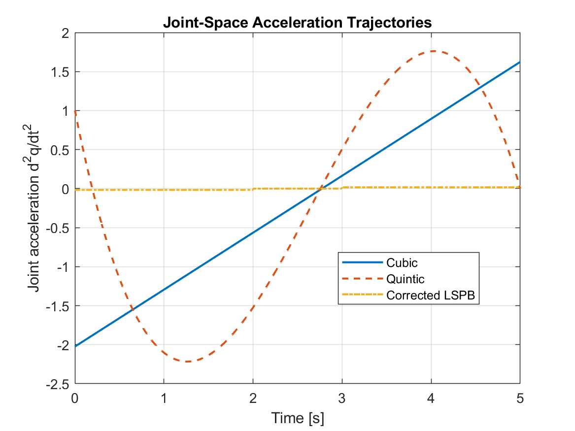
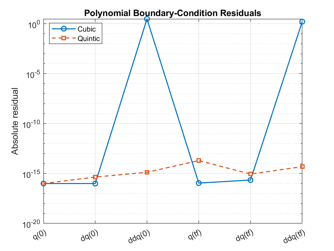
The cubic trajectory uses four coefficients and can satisfy only four independent endpoint constraints. In this project it enforces position and velocity at both endpoints, so it cannot also satisfy both specified accelerations. The quintic trajectory has six coefficients and can satisfy all six endpoint conditions.
| Boundary verification check | Result |
|---|---|
Cubic max residual for q and q̇ constraints | 2.220 × 10⁻¹⁶ |
Cubic acceleration mismatch at t = 0 | −3.024 |
Cubic acceleration mismatch at t = tf | +1.624 |
| Archived quintic closed-form formula | 9.500 × 10⁰ — FAIL |
Corrected quintic max q/q̇/q̈ residual | 1.987 × 10⁻¹⁴ |
The archived closed-form quintic coefficient expressions do not satisfy the stated boundary-value problem. The public version therefore solves the six boundary equations directly to recover a mathematically correct quintic trajectory while preserving the original endpoint conditions.
Position trajectories
Velocity trajectories
Acceleration trajectories
Polynomial jerk comparison
Boundary-condition residuals
Position–velocity phase plane
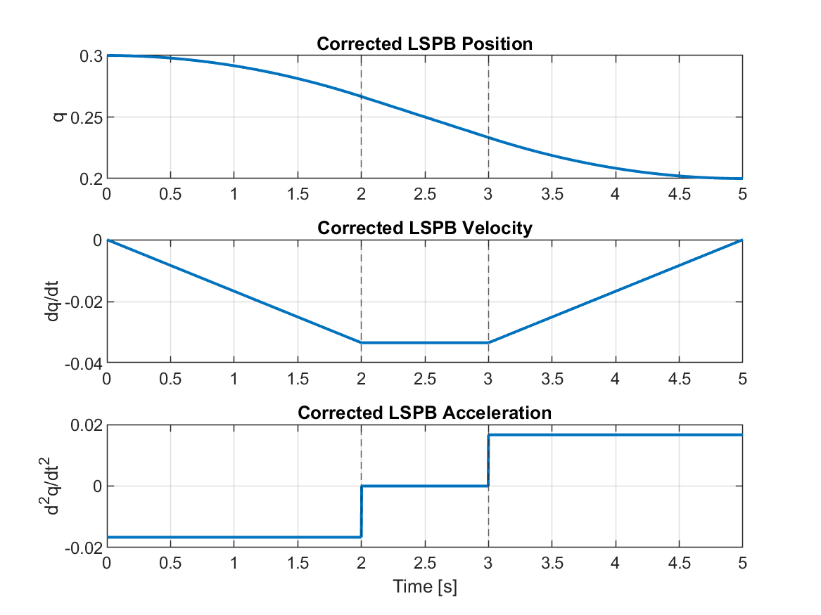
Corrected LSPB construction
The archived LSPB fragment used a positive cruise velocity even though the requested displacement was from 0.3 down to 0.2. That makes the original blend and cruise segments inconsistent. Keeping the source-derived blend time ta = 2 s, the cleaned implementation computes the only symmetric rest-to-rest LSPB cruise velocity that makes the trajectory continuous.
| Corrected LSPB quantity | Value |
|---|---|
Blend time, ta | 2.0 s |
Corrected cruise velocity, vc | −0.033333333 |
| Blend acceleration | −0.016666667 |
| Rest-to-rest continuity residual | 0.000 × 10⁰ |
Trajectory-shape metrics
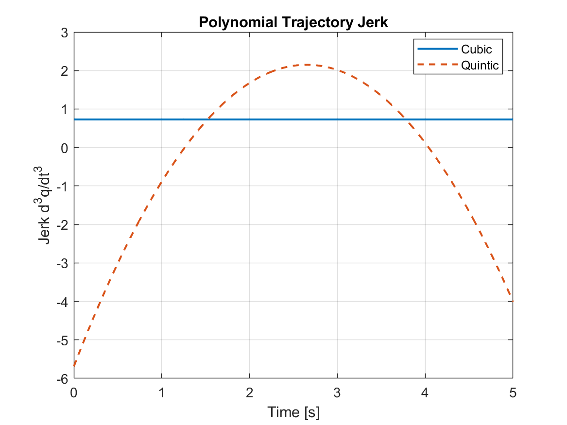
The following quantities are trajectory-shape metrics, not actuator-energy measurements. They help compare how aggressively each trajectory varies in velocity, acceleration, and jerk.
| Metric | Cubic | Corrected quintic | Corrected LSPB |
|---|---|---|---|
| Peak |q̇| | 2.0000 | 2.0940 | 0.0333 |
| Peak |q̈| | 2.0240 | 2.2165 | 0.0167 |
| ∫ q̈² dt | 5.7450 | 10.0928 | 0.0011 |
| ∫ q⃛² dt | 2.6616 | 22.9800 | — |
These values should not be used to declare one trajectory family universally superior. The corrected LSPB solves a different endpoint problem than the polynomial trajectories, and the polynomial endpoint conditions themselves force reversal and overshoot.
Scope and limitations
This is a single-joint trajectory-generation study, not a full manipulator path planner. There are no joint limits, collision constraints, actuator limits, or torque-level dynamic models. The cleaned repository emphasizes mathematical validation: it shows what the original cubic setup can satisfy, corrects the quintic boundary-value construction, and repairs the inconsistent LSPB sign convention.
Reproducibility
The public repository contains one self-contained MATLAB runner that reproduces all results, figures, coefficient exports, and boundary-verification tables without requiring external toolboxes. The generated outputs were validated in MATLAB R2022b.