Physics-Guided Identification of Nonlinear Thermal Dynamics
Physics-guided thermal system identification with a frozen synthetic extrapolation benchmark, multi-mechanism experiments, practical identifiability analysis, and KIT measured-room development studies.
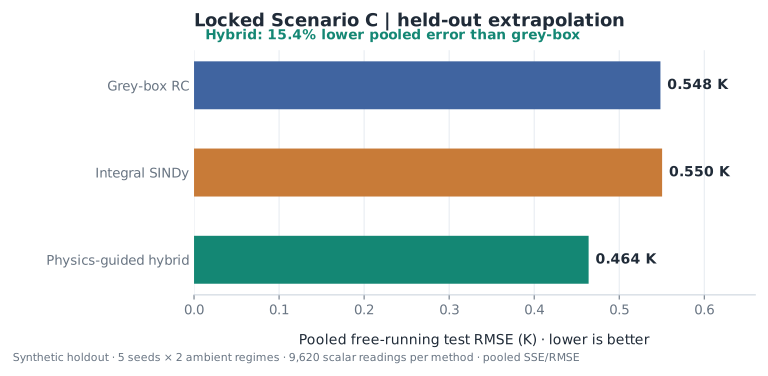
This independent Python research project investigates system identification when a physical model is useful but incomplete. I built a two-node thermal simulation with noisy feedback-controlled heating and nonlinear radiative heat loss, then compared three approaches: a constrained grey-box RC model, integral-form sparse identification of nonlinear dynamics (SINDy), and a physics-guided hybrid that augments a conserved energy-balance model with one passive, learned nonlinear heat-loss term.
The original benchmark result comes from a previously frozen, one-time synthetic held-out extrapolation test: the hybrid achieved 0.4640 K pooled temperature-prediction RMSE, compared with 0.5485 K for grey-box and 0.5504 K for SINDy. The approximately 15.4% reduction relative to grey-box is meaningful within this benchmark, but the development experiments also show several conditions in which the simpler grey-box model performs better.
Research scope: the original locked benchmark uses synthetic measurements; subsequent development research includes five synthetic missing-physics families and real room-level measurements from the KIT Living Lab Energy Campus. The measured-data extension is a separate, partially observed thermal model, not validation of the original two-measured-state simulator. The work is independent and is not an institutional collaboration or peer-reviewed publication. The source repository is currently private.
Research question
A nominal physics-based model often predicts well near its calibration regime, even if it omits a physical mechanism. A flexible data-driven model may represent nonlinear effects but can suffer from noisy observations, poorly conditioned features, and extrapolation outside the training temperatures. The research question is: can a small, physically constrained nonlinear residual improve predictive generalization without discarding the underlying conservation structure?
To examine this, the study evaluates not only prediction accuracy but also practical identifiability, excitation design, closed-loop sensor noise, training-data scarcity, operating-regime selection, and a locked final extrapolation protocol. A separate development-stage analysis explicitly checks situations where additional model complexity fails to help.
Thermal plant and missing physics
The simulated plant consists of two thermal capacitances connected by a thermal resistance, with heater input applied to node 1 and heat exchange with ambient air at node 2. The nominal energy-balance dynamics are:
C₁ · dT₁/dt = u − (T₁ − T₂)/R₁₂
C₂ · dT₂/dt = (T₁ − T₂)/R₁₂ − (T₂ − Tₐ)/R₂ₐ
The nonlinear synthetic truth adds a radiative heat-loss mechanism to the second equation:
qrad = εσA (T₂⁴ − Tₐ⁴)
C₂ · dT₂/dt = (T₁ − T₂)/R₁₂ − (T₂ − Tₐ)/R₂ₐ − qrad
| True simulation parameter | Value |
|---|---|
| Node 1 thermal capacitance, C₁ | 500 J/K |
| Node 2 thermal capacitance, C₂ | 2000 J/K |
| Inter-node resistance, R₁₂ | 0.4 K/W |
| Nominal ambient resistance, R₂ₐ | 0.8 K/W |
| Radiative emissivity, ε | 0.85 |
| Radiating area, A | 0.20 m² |
| Sampling interval | 60 s |
| Sensor noise standard deviation in final test | 0.08 K |
Radiative temperatures are in absolute kelvin. The values above define an illustrative simulated plant, not estimated material properties. Importantly, the fitted models do not receive the hidden radiation formula, emissivity, radiating area, or noise-free latent states. They use the two measured temperatures, the recorded applied heater power, and the ambient temperature.
Identification methods
Grey-box RC. The baseline preserves the nominal two-node energy-balance structure and fits four positive parameters, C₁, C₂, R₁₂, and R₂ₐ, through bounded simulation-error least squares. It uses exact zero-order-hold propagation of the nominal linear model. The omitted radiation can be partly absorbed into its estimated effective ambient conductance near the training regime.
Integral SINDy. The sparse model uses a fixed seven-feature library containing a constant, normalized temperature differences, heating power, and quadratic temperature terms. It estimates the dynamics through integrated windows rather than differentiating noisy measurements directly. For the Scenario C comparisons, the window is 24 samples, the stride is 4, and the sparsity threshold is 5 K/hour. Free-running predictions use numerical integration without intermediate measurement corrections.
Physics-guided hybrid. The hybrid retains the RC energy balance, but adds a learned signed-quadratic ambient heat-loss term:
qres = γ (T₂ − Tₐ) |T₂ − Tₐ| / (20 K), γ ≥ 0
The nonnegative constraint makes the residual passive with respect to the node-to-ambient temperature difference: its heat-flow direction does not oppose dissipation under the model's sign convention. This feature is not the true Stefan–Boltzmann radiation expression. The additional coefficient γ is fitted together with the four RC parameters and introduces flexibility as well as potential identifiability problems.
One-time held-out evaluation
The final evaluation protocol was frozen before accessing the reserved Scenario C test trajectories. It keeps all three model families and their hyperparameters unchanged. Each model is fitted using only four eight-hour training trajectories per seed replication, with stronger ±20 W pseudorandom binary sequence (PRBS) heating excitation.
| Protocol element | Locked configuration |
|---|---|
| Training ambient temperatures | 18, 20, 22, and 19°C |
| Training excitation | ±20 W PRBS |
| Training budget | 4 trajectories × 8 hours per replication |
| Held-out ambient temperatures | 12 and 28°C |
| Held-out excitation | ±12 W PRBS |
| Independent PRBS/noise seed replications | 5 |
| Held-out test trajectories | 10 (2 ambient regimes × 5 seeds) |
| Prediction method | Free-running replay of recorded heater power and ambient conditions |
| Initial condition | First noisy, measured two-temperature state |
| Primary metric | Pooled RMSE across both sensors and all held-out samples |
After the initial measured temperature, no future measurements are fed back into the prediction. The final scoring aggregates squared prediction errors before taking the square root. Each method contributes 9,620 scalar test observations. Those samples are correlated in time and come from only two distinct thermal operating environments; their count must not be confused with an independent sample size.
Final held-out prediction results
| Model | Pooled test RMSE | Completed replications |
|---|---|---|
| Grey-box RC | 0.548451 K | 5/5 |
| Integral SINDy | 0.550424 K | 5/5 |
| Physics-guided hybrid | 0.464001 K | 5/5 |
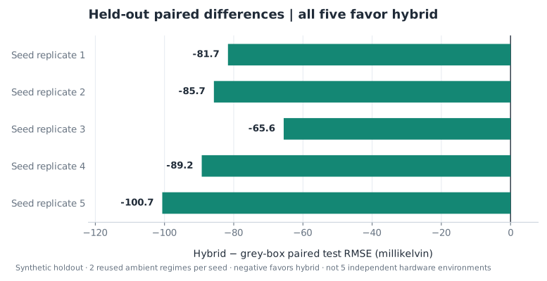
Extrapolation across ambient regimes
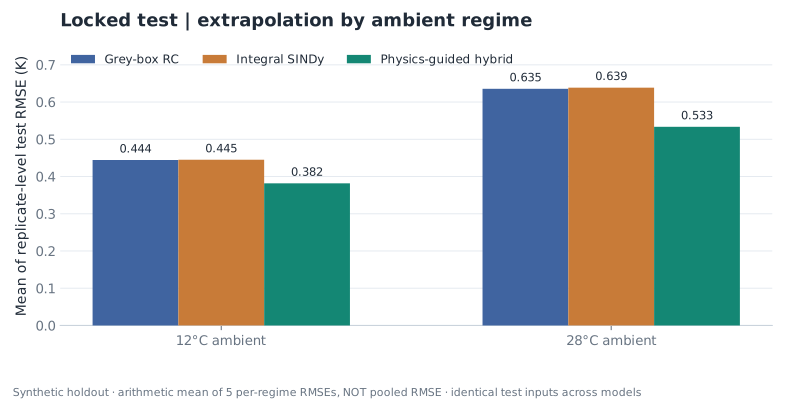
| Model | 12°C test regime | 28°C test regime |
|---|---|---|
| Grey-box RC | 0.4443 K | 0.6355 K |
| Integral SINDy | 0.4450 K | 0.6385 K |
| Physics-guided hybrid | 0.3816 K | 0.5335 K |
All three methods predict the unseen ambient regimes less accurately than the nearer-range development validation trajectories, where errors were typically near 0.09–0.10 K. The result therefore supports relative improvement under extrapolation, not uniformly small absolute prediction error.
Practical identifiability and excitation design
The fitted hybrid parameters are not automatically physically interpretable. The linear ambient heat-loss conductance, g = 1/R₂ₐ, and nonlinear coefficient γ can compensate for each other over a restricted temperature span. In a local Scenario B training-only analysis, their nuisance-adjusted sensitivity directions had a cosine of approximately 0.991, and the full five-parameter logarithmic sensitivity matrix had condition number approximately 388.
A profiled training-error analysis confirmed that moderately different γ values can be accommodated by changes in fitted R₂ₐ at very small increases in training error. This shows weak practical distinguishability under the tested conditions, not proven structural non-identifiability or a calibrated parameter confidence interval.
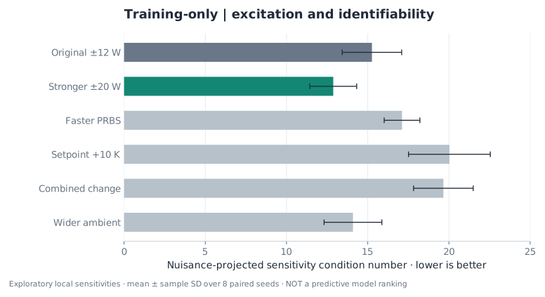
A crossed development validation experiment then separated the effects of more informative training excitation from more demanding evaluation inputs. When each fitted method was evaluated on exactly the same ±12 W validation inputs, training with stronger excitation decreased mean prediction error for all three methods: from 0.09461 to 0.09373 K for grey-box, 0.09786 to 0.09597 K for SINDy, and 0.09711 to 0.09688 K for hybrid. Grey-box still had the lowest error on these nearer validation regimes.
Data availability and operating-regime sensitivity
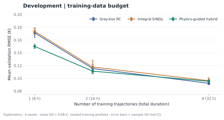
A multi-seed training-budget study explored how the models behave with only one, two, or four complete eight-hour training trajectories. When training budgets used nested prefixes of the available operating regimes, the hybrid performed best with one or two trajectories, whereas grey-box achieved the lowest mean error with four.
| Training trajectories | Grey-box RMSE | SINDy RMSE | Hybrid RMSE |
|---|---|---|---|
| 1 (8 hours) | 0.17118 K | 0.17352 K | 0.14997 K |
| 2 (16 hours) | 0.11527 K | 0.11769 K | 0.11122 K |
| 4 (32 hours) | 0.09216 K | 0.09618 K | 0.09529 K |
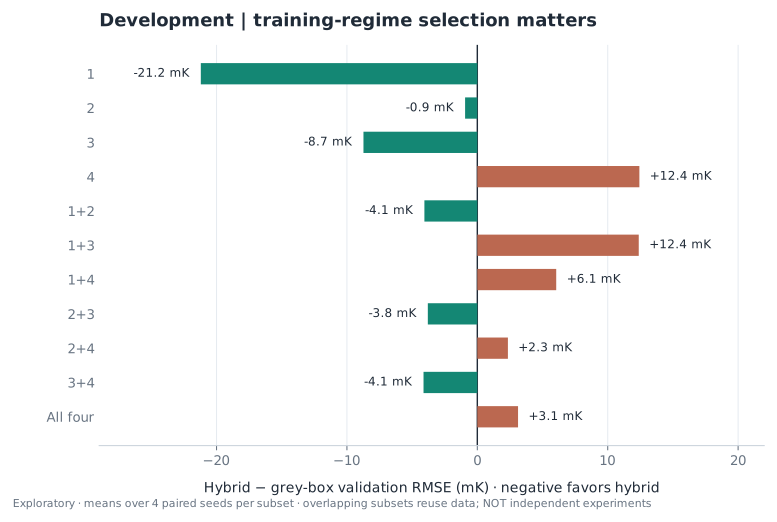
To test whether that low-data advantage was an artifact of always choosing the first training regimes, the next analysis exhausted all four singleton and six two-trajectory subsets, plus the complete four-trajectory set. The result changed with operating-condition selection: hybrid beat grey-box in 11/16 seed/subset comparisons for singletons but only 12/24 for pairs. In the fourth training regime alone, grey-box won all four seed replications.
Sensor-noise robustness
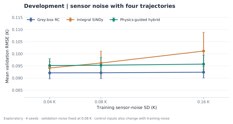
At the four-trajectory training budget, a noise sweep increased the standard deviation of training sensor measurements from 0.04 K to 0.16 K, while validation sensor noise remained 0.08 K. Mean SINDy validation error increased more strongly than grey-box or hybrid error.
| Training noise SD | Grey-box RMSE | SINDy RMSE | Hybrid RMSE |
|---|---|---|---|
| 0.04 K | 0.09214 K | 0.09414 K | 0.09515 K |
| 0.08 K | 0.09216 K | 0.09618 K | 0.09529 K |
| 0.16 K | 0.09240 K | 0.10112 K | 0.09573 K |
Additional synthetic research: model structure and missing physics
Following the original locked synthetic evaluation, I investigated whether the learned residual remains useful when the unmodelled mechanism changes. Five deliberately specified synthetic plant families covered nominal physics, radiation, nonlinear convection, internal-contact heat transfer, and unknown input/heater mismatch. A separate 30-configuration development cohort compared grey-box RC, passive and unconstrained nonlinear residuals, and a constant-load alternative. Always using the passive hybrid gave a mean RMSE of 0.22333 K versus 0.24337 K for grey-box, but validation-based selectors did not improve the cohort mean over always-passive.
An additional 15-configuration development study introduced a generic affine time-varying latent heat-load model. A four-class validation selector improved the mean score mainly in the unknown-load physics family: its aggregate mean advantage relative to always-passive was approximately 0.05389 K, with essentially the entire improvement attributable to that family. These cohorts have different candidate model sets and cannot be described as an identical-method replication or a final independent paper test.
Measured thermal data: KIT Building 3
To investigate the challenges beyond simulation, I used public measurements from the KIT Living Lab Energy Campus dataset. The data include measured room-air temperature, room-level signed hydronic thermal power, outdoor temperature and solar irradiance, together with hydronic flow and supply/return water temperatures. I verified source-file checksums, aligned timestamps, preserved negative power readings, and examined data gaps. The model for these measurements uses one observed room temperature and one unobserved thermal-mass/wall state; a neighboring room is not treated as a directly measured wall temperature.
For this real-data development study, I fitted positive-parameter RC models with training-only latent-wall initialization, then compared uninterrupted 12-hour conditional-input predictions at a common forecast origin. The predictions replay recorded future heating power and weather, rather than forecasting these external inputs in advance. Both positive and negative modelling outcomes were preserved.
| Development model / 12-hour RMSE | KIT Building 3 R1 | KIT Building 3 R4 |
|---|---|---|
| Persistence at training boundary | 1.117 °C | 0.412 °C |
| Grey-box latent-wall RC | 0.330 °C | 0.259 °C |
| Passive nonlinear wall-loss extension | 0.319 °C | 0.246 °C |
| Fitted first-order radiator heat-delivery delay | 0.588 °C | 0.325 °C |
These values come from a later, non-overlapping development window of KIT Experiment 1, not an independent building or final confirmatory test. In an earlier Experiment 1 development window, the passive model was slightly worse than grey-box for R1 and failed to converge for R4; the latter failure is not concealed. The fitted radiator time constants in the later window reached their imposed lower bounds, and physical parameter estimates showed boundary and confounding problems. The real KIT results are consequently mixed, not evidence that the hybrid consistently outperforms simpler models in real buildings.
The KIT data are attributed to their original authors. Only Experiment 1 was used for fitted measured-data development. Experiment 2 was not used for model confirmation, and no additional independent real-building validation or calibrated parameter-recovery claim is made.
Reproducibility and verification
The Python implementation contains the thermal simulator, deterministic dataset specifications, model-fitting procedures, training/validation experiments, model-comparison scripts, automated tests, and versioned numerical evidence. The one-time final test ran under a frozen protocol in GitHub Actions; its results were saved without subsequent model retuning.
The full repository read-only quality audit reached 218 passing automated tests as of 14 November 2026. Earlier clean-checkout checks verified the original benchmark with 98 tests. It compiled the Python source and independently recomputed the reported final pooled RMSE values from committed squared-error totals and sample counts—without regenerating the held-out trajectories. Seven vector figures were generated from those saved results and checked against source-file hashes. The project repository and full technical report are currently private; the verified figures and principal results are reproduced here so the scientific record can be assessed without repository access.
Scope and limitations
The final evaluation uses a single simulated nonlinear heat-transfer mechanism and only two distinct ambient test regimes, repeated over five noise/excitation seeds. The 9,620 scalar observations per model are correlated time samples, not 9,620 independent physical cases. The fitted hybrid residual is a useful signed-quadratic approximation in the tested setup but is not the true radiation equation, and its coefficient is practically confounded with linear ambient conductance.
The work does not establish independent real-building or hardware generalization, experimental sensor calibration, accurate recovery of unique physical coefficients, model-based closed-loop stability with the identified dynamics, calibrated statistical confidence intervals, or general superiority of the hybrid over simpler identification approaches. The stronger held-out outcome should be read together with the negative and mixed development findings rather than as a universal performance claim.
Research perspective
The main lesson is methodological: physics-guided flexibility can help extrapolation, but only when evaluated against strong baselines with explicit data separation and identifiability checks. Subsequent work extended the study to multiple synthetic mechanisms and measured KIT development data; the resulting model-selection tradeoffs and negative cases are documented above. A future journal study would still require a precisely differentiated research contribution and a new independent confirmatory protocol. The existing repository is being preserved as a completed research portfolio project rather than presented as a published paper.