Nonlinear Vehicle Dynamics, Tire-Force Modeling & Linearization
MATLAB project for five-state nonlinear vehicle dynamics, combined-slip tire-force modeling, tire saturation, straight-line operating-point linearization, and nonlinear-versus-linear analysis.
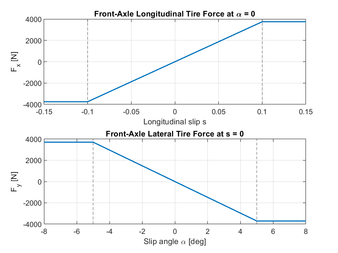
This MATLAB project studies a five-state nonlinear planar vehicle model with front steering, front and rear wheel rotational dynamics, longitudinal and lateral tire slip, combined-slip force coupling, and tire-force saturation. I reorganized the archived Advanced Control work into one reproducible analysis workflow that makes the model assumptions, operating point, linearization, and nonlinear effects easier to inspect.
The complete implementation and generated results are available here: GitHub repository
The archived source contained useful vehicle and tire equations, but it also depended on a missing saturation helper and used a substituted state/input point that was not a consistent straight-line equilibrium. The public version keeps the original five-state model and parameter set, replaces the missing saturation operation explicitly, and linearizes numerically around a physically consistent 15 m/s straight-line operating point.
Vehicle and tire model
The state vector is x = [Vx, Vy, r, ωf, ωr]ᵀ, containing longitudinal velocity, lateral velocity, yaw rate, and front/rear wheel angular speed. The input vector is u = [δ, Tf, Tr]ᵀ, containing front steering angle and front/rear wheel torques.
| Model parameter | Value |
|---|---|
| Vehicle mass, m | 1000 kg |
| Yaw inertia, Iz | 2000 kg·m² |
| Wheel inertia, Iw | 30 kg·m² |
| CG to front axle, a₁ | 1.35 m |
| CG to rear axle, a₂ | 1.50 m |
| Wheel radius, R | 0.35 m |
| Front/rear lateral tire coefficients | 8.5 / 8.5 |
| Front/rear longitudinal tire coefficients | 7.5 / 7.5 |
| Longitudinal-slip limit | ±0.10 |
| Slip-angle limit | ±5° |
The slip definitions follow the archived model. Front and rear slip angles depend on lateral velocity and yaw rate, while longitudinal slip compares wheel circumferential speed with vehicle longitudinal speed. The tire-force law couples longitudinal and lateral behavior: increasing slip angle reduces available longitudinal force, and increasing longitudinal slip reduces available lateral force.
Tire-force characteristics
The saturation operation is not an added tire-control algorithm. It replaces the missing my_saturation.m helper referenced by the archived source and makes the original force-limiting assumption explicit and reproducible.
Combined-slip coupling
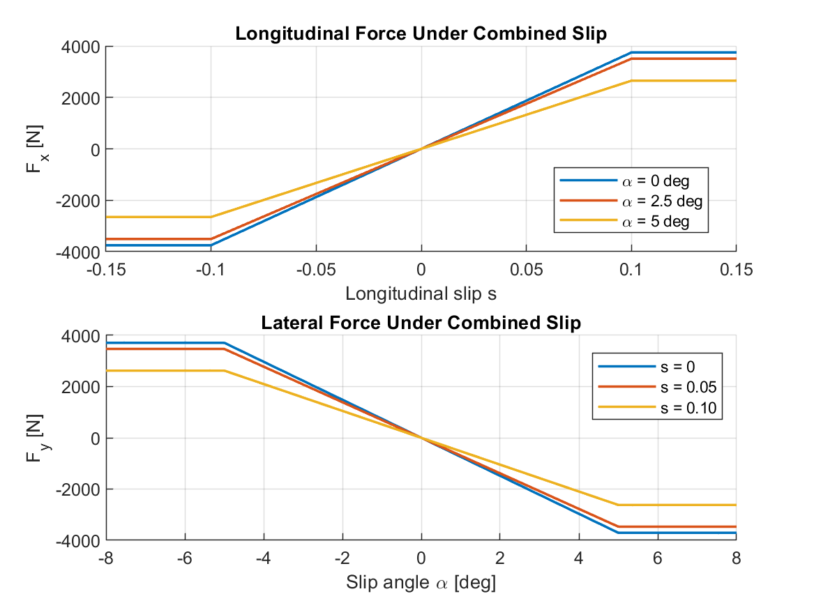
This is a compact academic combined-slip model retained from the original coursework. It is useful for studying nonlinear coupling and saturation, but it is not presented as a manufacturer-calibrated Magic Formula/Pacejka tire model.
Straight-line operating point and linearization
For the cleaned linear analysis, I use a consistent straight-line operating point at 15 m/s (54 km/h): zero lateral velocity, zero yaw rate, zero steering, zero wheel torque, and front/rear wheel speeds equal to the rolling speed Vx/R. The nonlinear state derivative is exactly zero at this point for the implemented model.
| Operating-point / linear-model check | Result |
|---|---|
| Longitudinal speed | 15.0 m/s (54.0 km/h) |
| Front/rear wheel speed | 42.8571 rad/s |
| Equilibrium residual ‖f(x₀,u₀)‖₂ | 0.000e+00 |
| State dimension | 5 |
| Input dimension | 3 |
| Controllability rank | 5 / 5 |
The Jacobian matrices A and B are evaluated using central finite differences around this operating point. This avoids a Symbolic Math Toolbox dependency and gives a directly reproducible local linear model.
Small-signal nonlinear versus linear response
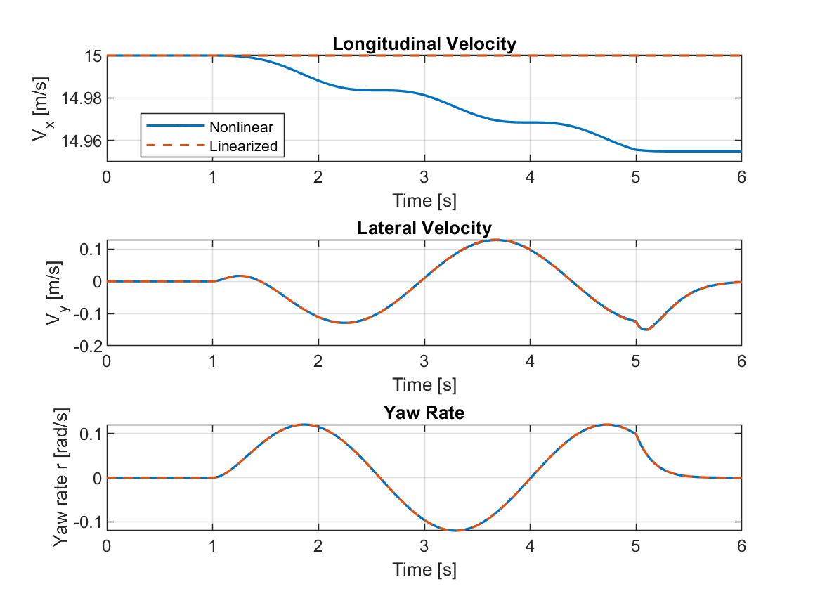
| Small-signal comparison metric | RMSE |
|---|---|
| Longitudinal velocity, Vx | 0.027043 m/s |
| Lateral velocity, Vy | 6.862 × 10⁻⁴ m/s |
| Yaw rate, r | 1.088 × 10⁻⁴ rad/s |
| Front wheel speed | 0.075419 rad/s |
| Rear wheel speed | 0.075419 rad/s |
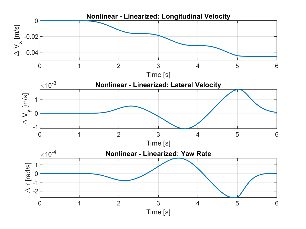
The largest discrepancy is in longitudinal velocity. That is expected here because steering-induced longitudinal effects enter through nonlinear force projection and are not fully represented by the first-order straight-line linearization. The small-signal case remains well within the tire saturation region: the maximum raw slip angle is approximately 1.145° and the maximum raw longitudinal slip is approximately 1.37 × 10⁻⁴.
Linearization error
Larger-steering nonlinear behavior
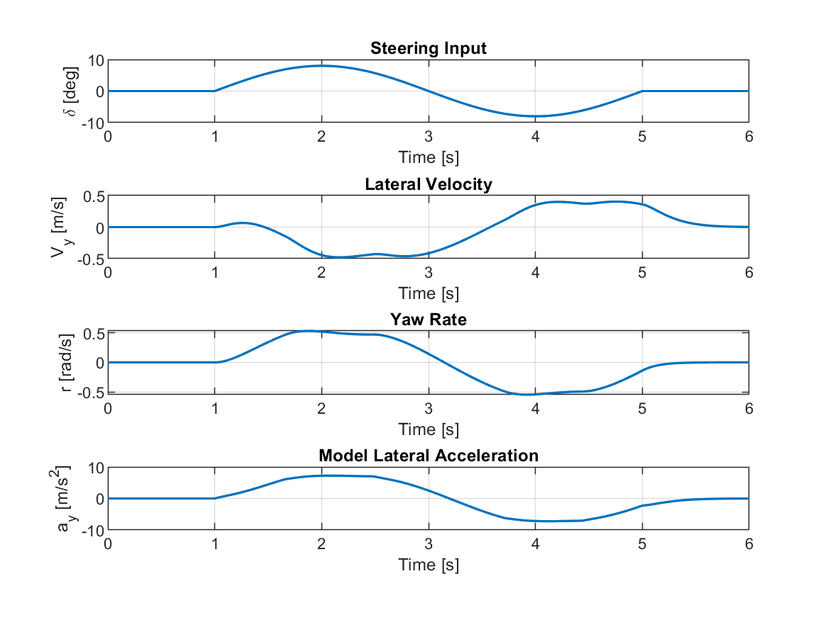
| Larger-steering metric | Value |
|---|---|
| Maximum raw slip angle | 7.105° |
| Maximum raw longitudinal slip | 0.004607 |
| Samples with slip-angle saturation | 25.9% |
| Samples with longitudinal-slip saturation | 0% |
| Maximum model lateral acceleration | 7.240 m/s² |
| Maximum longitudinal-speed reduction | 1.067 m/s |
These values characterize the implemented simulation only. In particular, the 7.240 m/s² lateral-acceleration value should not be interpreted as a validated handling limit for a physical vehicle.
Tire slip and saturation
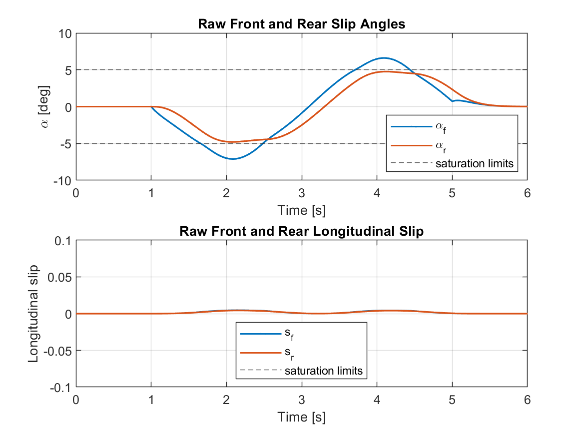
The plotted curves are the raw kinematic slip variables. The tire-force equations evaluate their saturated versions. Keeping these two quantities separate makes it clear when the model is entering the imposed nonlinear force-limiting region.
Linearized-model eigenvalues
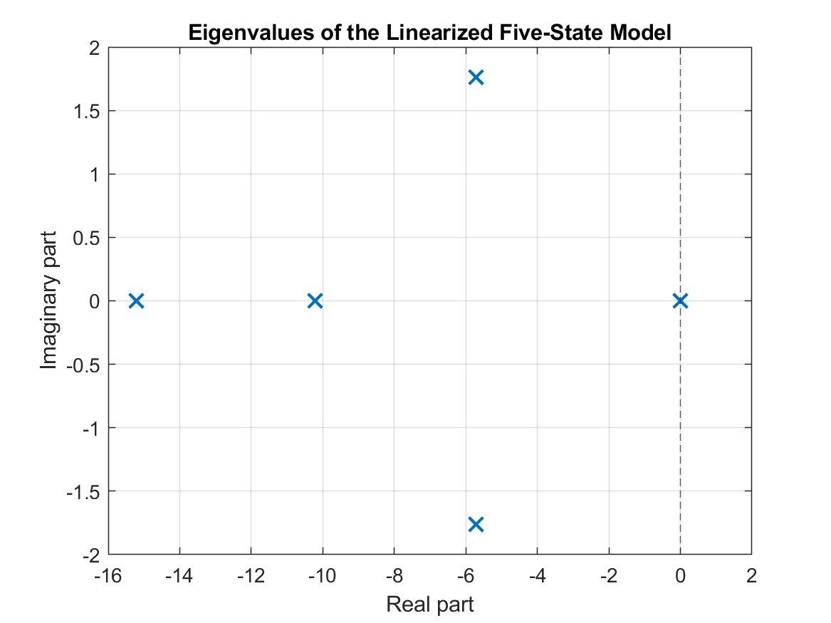
| Linearized-model eigenvalue |
|---|
| 0 |
| −15.2083 |
| −5.7180 + 1.7591j |
| −5.7180 − 1.7591j |
| −10.2083 |
The near-zero longitudinal mode is consistent with this simplified straight-line model because aerodynamic drag, rolling resistance, and a longitudinal-speed regulator are not included. The figure therefore should not be read as evidence of a complete road-vehicle stability analysis.
Scope and limitations
This project is a simulation and model-analysis study. The tire coefficients and normal loads are preserved from the archived academic model rather than identified from experimental tire data. Dynamic load transfer, aerodynamic drag, rolling resistance, actuator dynamics, road-friction variation, and sensor noise are not modelled.
The numerical linear model is local to the documented 15 m/s straight-line operating point. The larger-steering experiment is included specifically to show where nonlinear/saturation effects become important; it is not an experimental validation of vehicle handling.
No closed-loop steering controller, yaw-stability controller, ABS, traction-control algorithm, or MPC is claimed in this repository. Those belong to separate control-design projects rather than this vehicle-modeling study.
Reproducibility
The repository contains a self-contained MATLAB runner, model notes, generated figures, the linearized A and B matrices, eigenvalues, CSV metrics, and a text summary. Running run_nonlinear_vehicle_project.m regenerates the complete analysis. The validated run was performed with MATLAB R2022b, and the cleaned runner does not require Simulink or the Symbolic Math Toolbox.