Mobile Robot Navigation Basics | Mohammad Hossein Fakouri

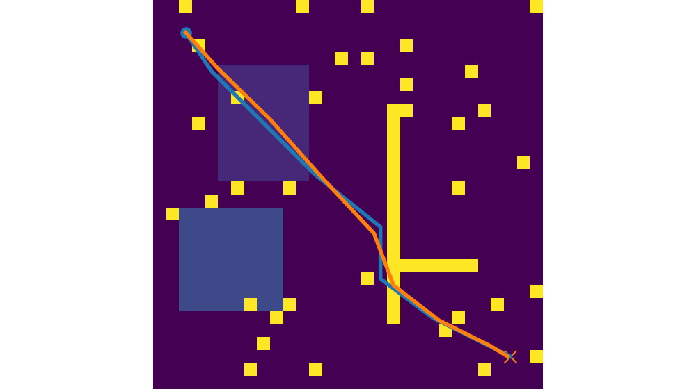
This is a small Python practice project that I made to understand some basic parts of mobile robot navigation. It is not a complete autonomous vehicle project. I made it more as a learning work, because I wanted to connect my control background with path planning and simple robot motion.

The project is available here: GitHub repository

The project starts from a small grid map, then a larger terrain map, then A* path planning, and finally a simple vehicle tracking model. After that, I added one small disturbed tracking test and some simple metrics.

Basic terrain grid

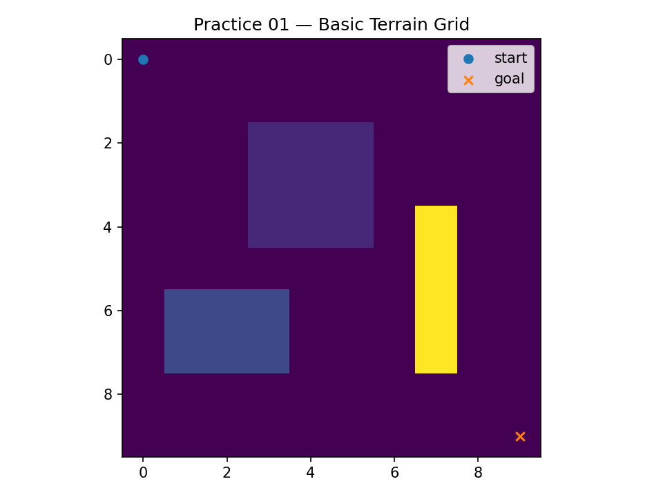
Basic 10 by 10 terrain grid with start and goal points — **Figure 1. Basic 10 by 10 terrain grid.** This first plot shows the small terrain map. The dark cells are normal terrain, the colored blocks are rough and risky areas, and the yellow block is an obstacle. The blue point is start and the orange cross is goal. Here I only checked if I can make a grid map and plot terrain types correctly.

The first step was a 10 by 10 NumPy grid. I used numbers for terrain types: 0 for flat terrain, 1 for rough terrain, 2 for risky terrain like snow or ice, and 9 for obstacle.

This was very simple, but useful for me. It also reminded me that NumPy indexing is row-column, not normal x-y coordinate. So (0, 0) appears at top-left.

Larger terrain map

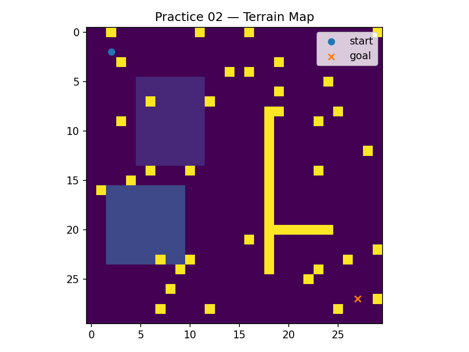
Larger 30 by 30 terrain map with random obstacles — **Figure 2. Larger terrain map with obstacles and terrain areas.** This plot shows the larger 30 by 30 map. I added rough terrain, risky terrain, obstacle walls, and random obstacle cells. The yellow cells are obstacles. This figure is still only the environment, not the robot motion.

After the small grid, I made a larger map. The random obstacles are not from real sensor data. I added them just to make the map less empty and more useful for planning practice.

I also used a fixed random seed, so the map stays same when I run the script again.

A* path planning

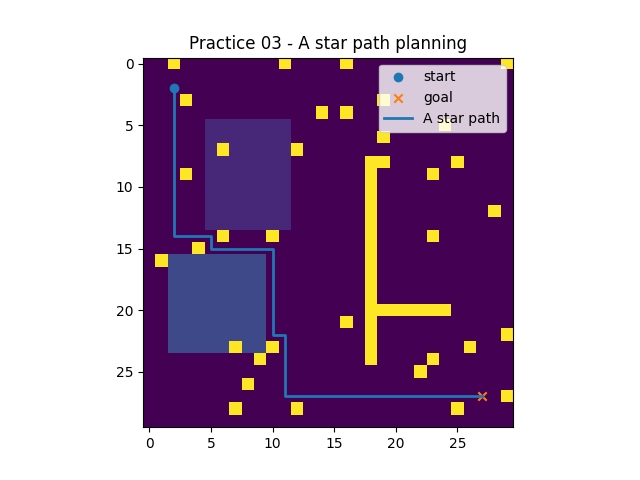
A star path planning result on terrain grid — **Figure 3. A* path planning on the terrain grid.** This figure shows the A* path on the terrain map. The blue line is the planned route from start to goal. The path avoids obstacles, and it also uses terrain costs. It is not smooth, because it is a grid path and I used only up, down, left, and right movements.

In this step I added A* path planning. The planner tries to find a route from start to goal. Flat cells have low cost, rough cells have more cost, risky cells have more cost, and obstacles have very high cost.

This part helped me understand that planning and control are not the same. A* gives a route, but it does not move the robot.

Simple vehicle tracking

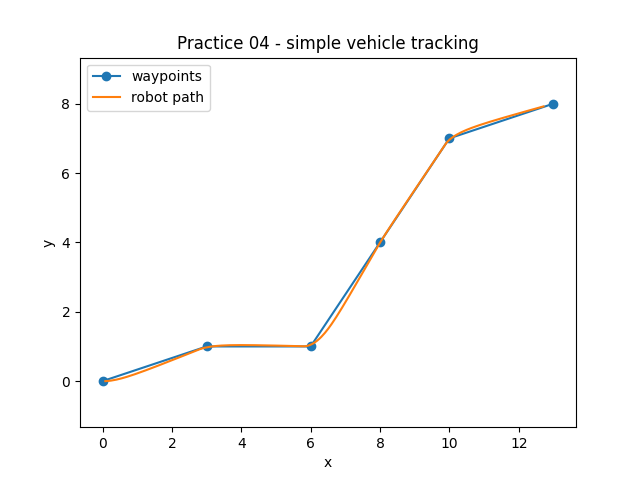
Before connecting the A* path to the map, I tested a simple vehicle model. I used a unicycle model with x, y, and theta.

This model is basic. It does not include wheel slip, acceleration limit, motor dynamics, or terrain effect. But it was enough for practicing heading-based tracking.

A* path with vehicle tracking

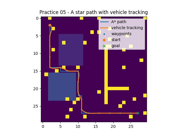
A star planned path connected to simple vehicle tracking — **Figure 5. A* planned path connected to vehicle tracking.** This plot connects the planner and vehicle tracking. The blue line is the A* path, the orange line is the simulated vehicle path, and the small points are selected waypoints. The vehicle path is close to the planned path, but not exactly same, because A* is discrete and the vehicle model is continuous.

Here I converted the A* path to waypoints for the vehicle model. A* gives points as row and column, but the vehicle model uses x and y.

x = column
y = row

I did not use every A* point as waypoint. I selected every few points, because the full path has many close cells and the simple vehicle would turn too much.

Disturbed tracking and simple metrics

Disturbed vehicle tracking on terrain map — **Figure 6. Vehicle tracking with small disturbance.** In this plot, I added a small random heading noise to the vehicle model. I also changed speed based on terrain type. The vehicle moves slower on rough and risky terrain. This is not a realistic winter terrain model, but it is a small test to see what happens when the motion is not perfect.

Tracking error during disturbed vehicle motion — **Figure 7. Tracking error during disturbed motion.** This plot shows the distance between the vehicle and the current target waypoint during simulation. The error changes because the vehicle is moving with heading noise and it can not follow the path perfectly. I used this plot only as a simple evaluation result.

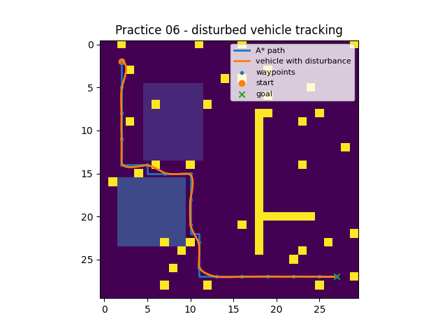
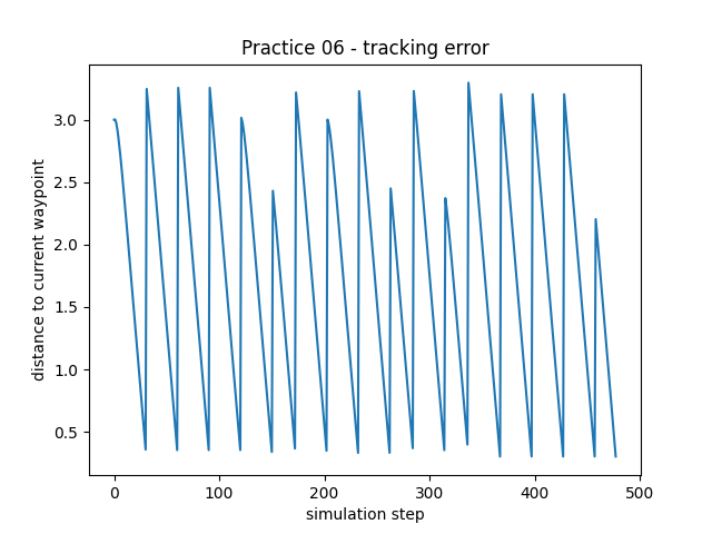
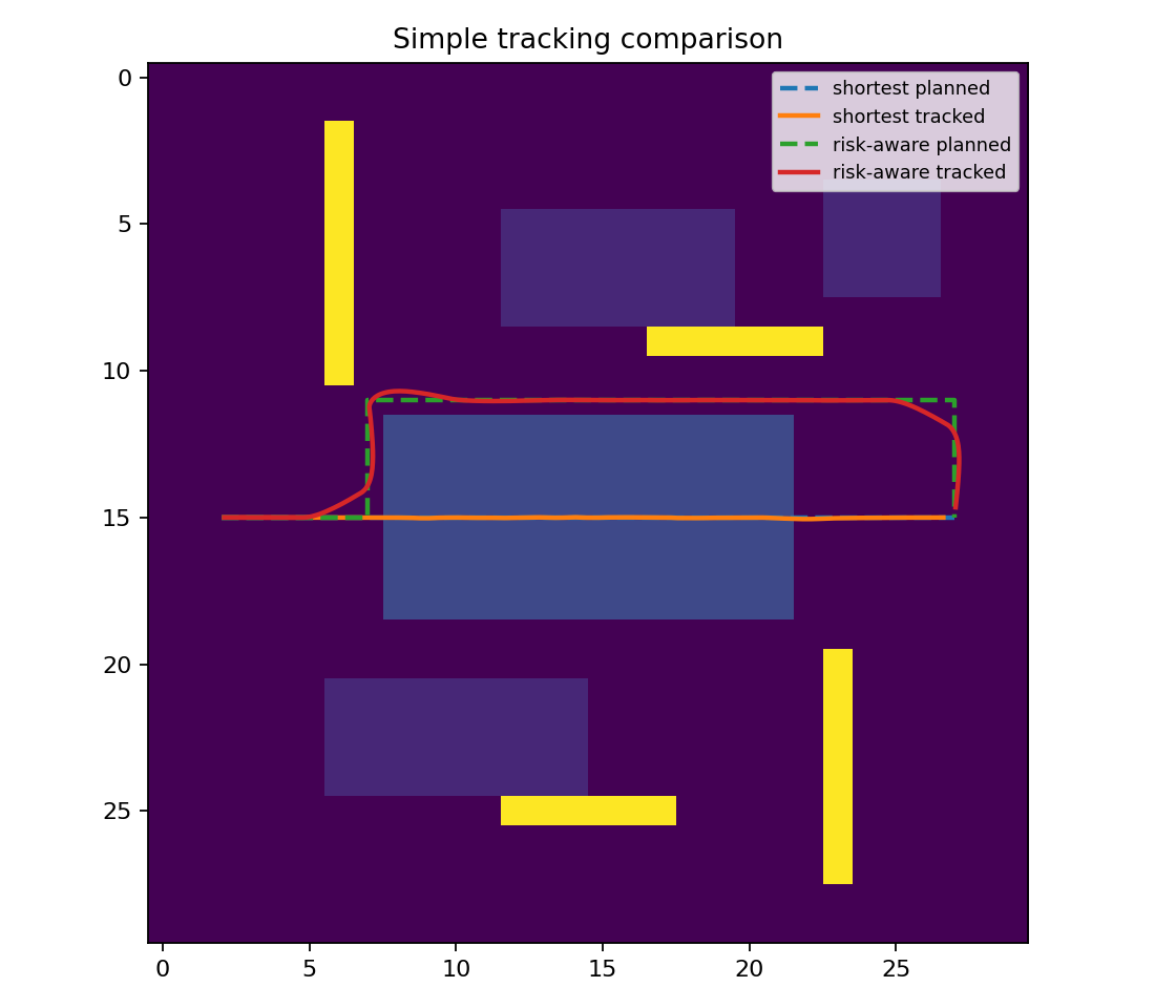
For the last part, I added a small disturbance test. The vehicle does not move in a perfect condition. I added random heading noise, and also terrain-dependent speed. This made the simulation a little more close to rough motion, but still it is very simple.

Metric	Value
A* path cells	51
Selected waypoints	18
Path cost	51.0
Rough cells in path	0
Risky cells in path	0
Mean tracking error	1.71
Maximum tracking error	3.30

In this run, the A* path did not pass through rough or risky cells, so both of them are zero. The mean tracking error was about 1.71 and the maximum tracking error was about 3.30. The error is not very small, but for this basic model it is acceptable.

Shortest path vs risk-aware planning

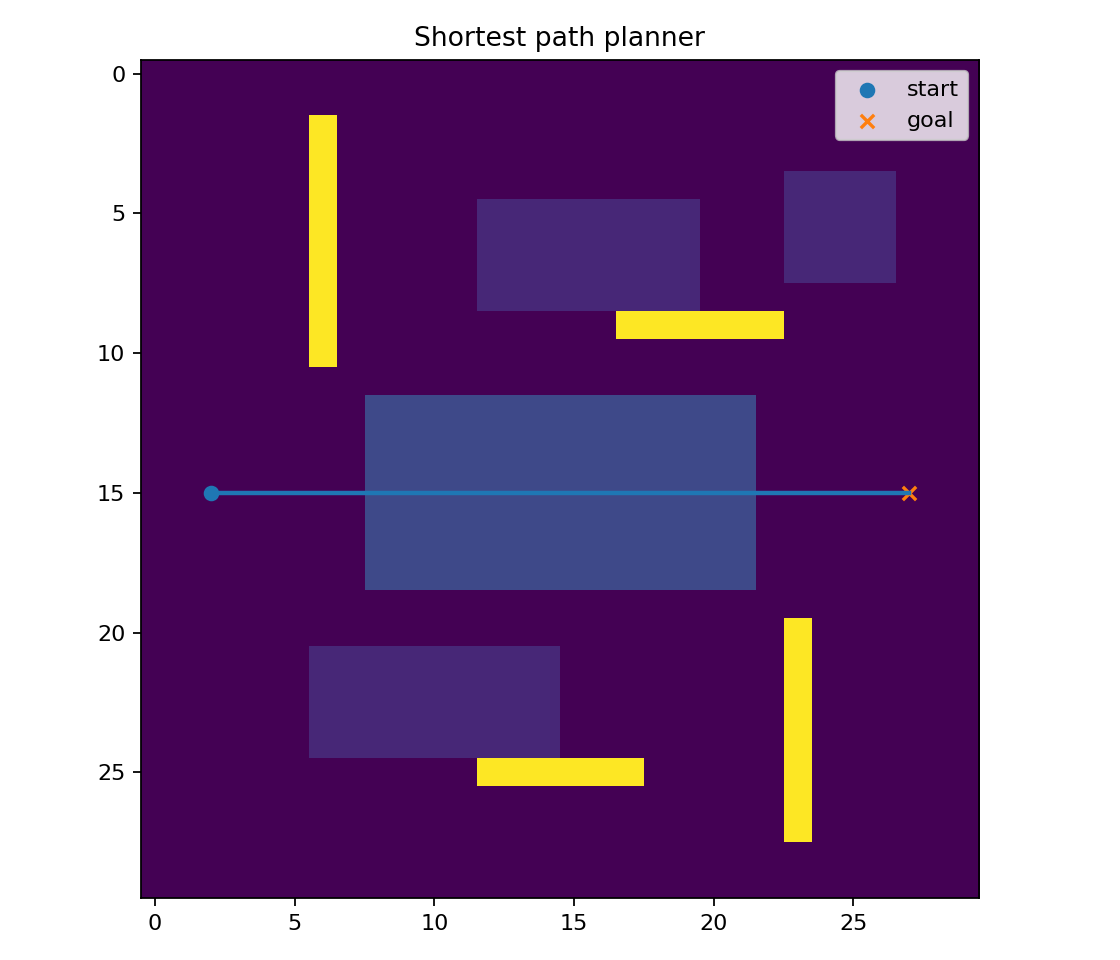
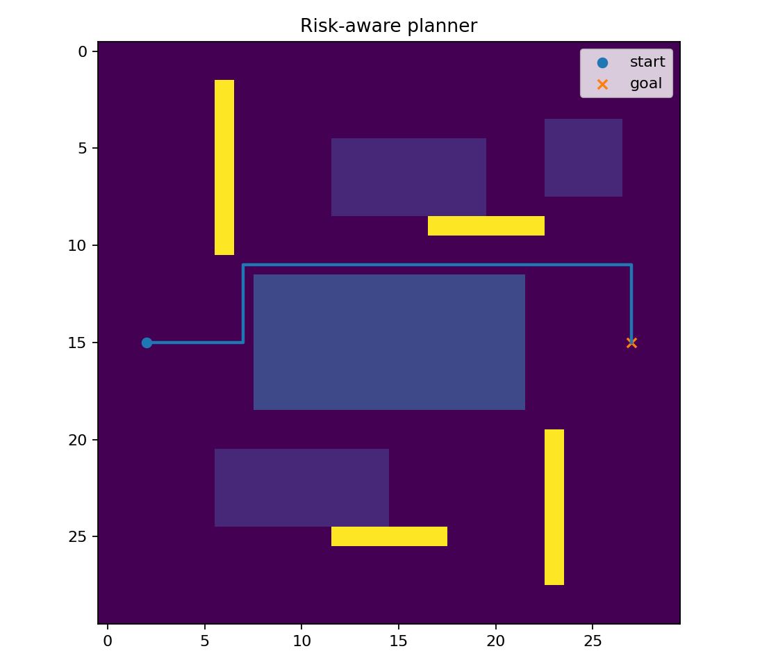
Shortest path planner on terrain grid — **Figure 8. Shortest path planner.** This planner tries to find the shorter route from start to goal. It does not care much about risky terrain, so the path crosses the risky area in the middle of the map.

Risk-aware path planner on terrain grid — **Figure 9. Risk-aware path planner.** This path is longer, but it avoid the risky cells. I changed the terrain costs, so risky terrain becomes expensive for the planner.

After the first A* tests, I wanted to compare two different planning ideas. The shortest path planner only tries to reduce the grid distance. The risk-aware planner uses distance and terrain cost together.

This is still a simple grid example. It is not a full autonomous driving system. But it shows one useful idea: in rough terrain, the shortest route is not always the best one.

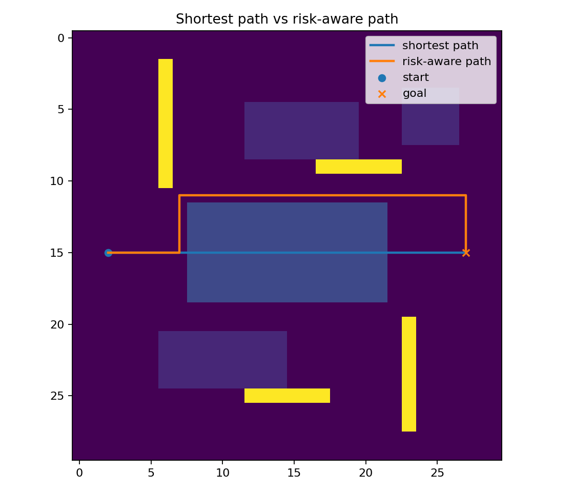
Shortest path and risk-aware path on the same terrain map — **Figure 10. Shortest path and risk-aware path on the same map.** The shortest path is more direct, but it crosses risky cells. The risk-aware path goes around the risky region and gives lower terrain cost.

Planner	Path length	Total terrain cost	Risk exposure	Tracking error	Success
Shortest path	25	179.0	14	1.81	Yes
Risk-aware path	33	33.0	0	1.71	Yes

The result is simple but useful. The shortest path has lower distance, but much higher terrain cost. It also passed through 14 risky cells. The risk-aware path was longer, but it had zero risky cells in this test.

Tracking comparison for shortest path and risk-aware path — **Figure 11. Tracking comparison for both planners.** I also used the same simple vehicle model to follow both paths. The tracking is not perfect, because the vehicle model has small noise and very basic dynamics.

What I learned

This project helped me understand the connection between terrain representation, path planning, and simple mobile robot movement.

The main things I practiced were:

making a terrain grid with NumPy,
using numbers for terrain types,
assigning simple costs for flat, rough, risky, and obstacle cells,
implementing a basic A* planner,
converting grid path to x-y waypoints,
simulating a simple vehicle model,
adding small disturbance and tracking error,
plotting the planned path and tracking path together.

There are still many limitation in this project. The map is manually created. There is no camera, no LiDAR, no ROS, no real robot, and no advanced controller. The terrain cost values are also manually selected.

But for a small practice work, it was useful for me. It gave me a first working example that connects map, planner, tracking, and simple evaluation. Later I can improve it by adding diagonal movement, path smoothing, animation, or maybe a ROS 2 version.