Inverted Pendulum: State-Space Analysis, LQR & Animation

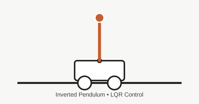
This MATLAB project studies stabilization of the classical cart–inverted-pendulum system around the upright equilibrium using continuous-time linear quadratic regulation. The cleaned version focuses on the engineering questions that matter most: whether the linearized system is controllable and observable, how the unstable open-loop poles move under feedback, and how changing the LQR input penalty changes settling time, control effort, and cart excursion.

The complete MATLAB implementation and generated numerical results are available here: GitHub repository

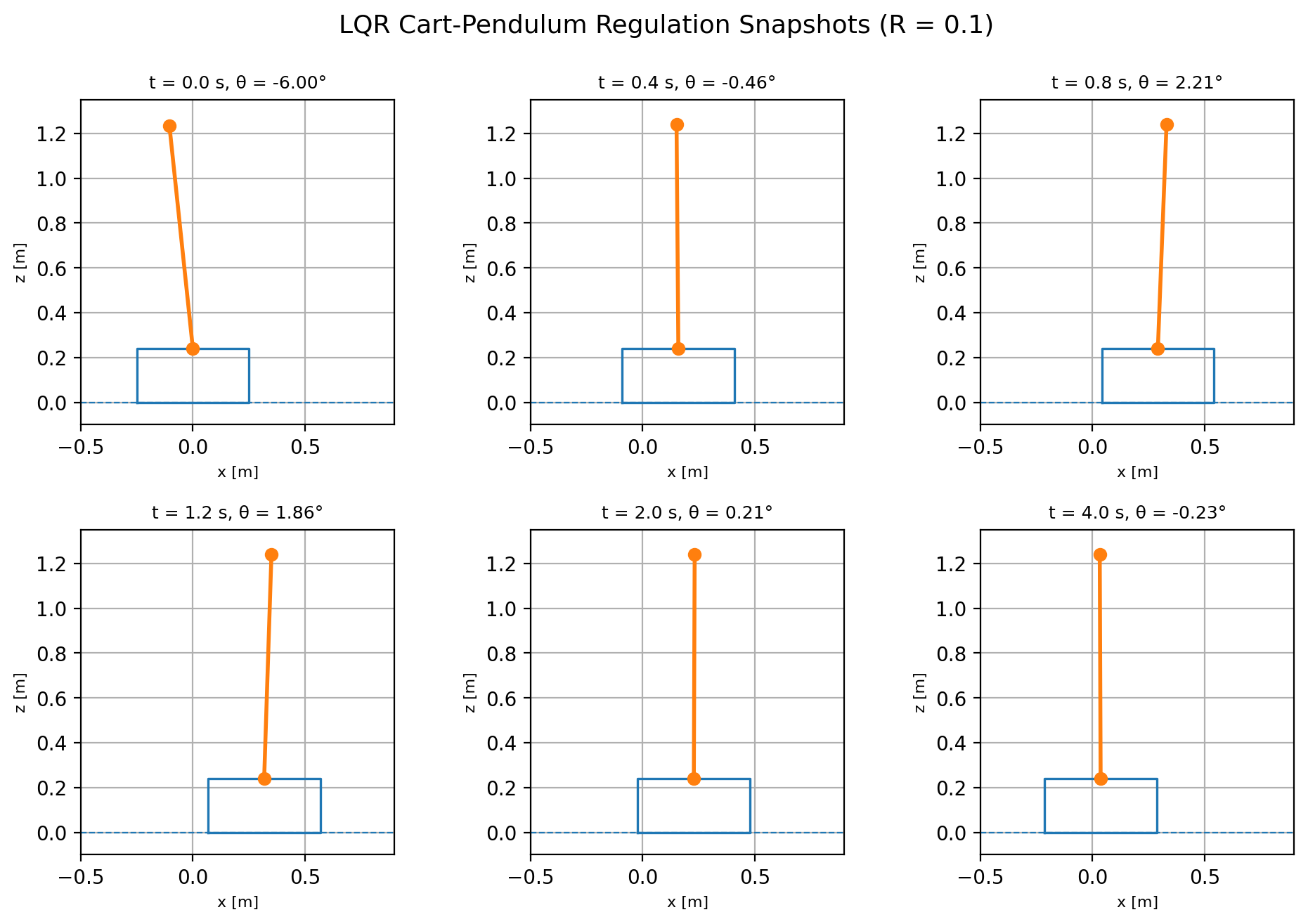
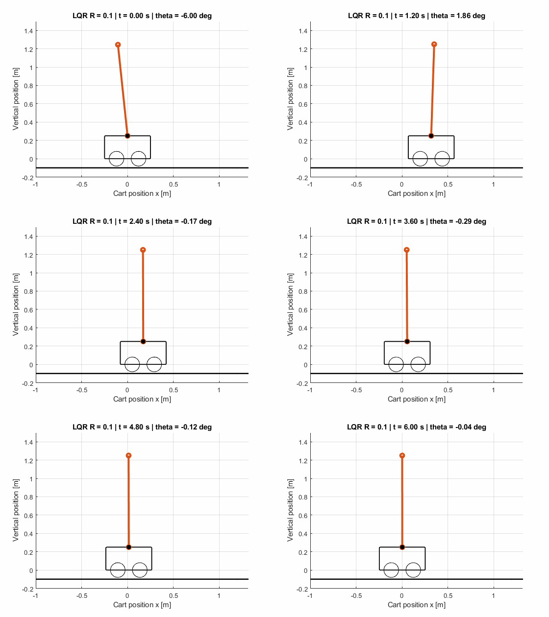
The public project is intentionally conservative about provenance. An archived Simulink animation model was not reused because its callback text contained attribution to another author. The cart–pendulum visualization shown here is generated from a new MATLAB animation written directly around the simulated cart position and pendulum angle.

Linear upright-equilibrium model

The state vector is x = [xc, θ, ẋc, θ̇]ᵀ, where xc is cart position and θ = 0 denotes the upright equilibrium. The model is the source-derived four-state linearization used in the original Modern Control work.

Physical parameter	Value
Cart mass, mc	1.5 kg
Pendulum mass, mp	0.5 kg
Pendulum length, L	1.0 m
Gravity, g	9.81 m/s²
Cart damping, d1	0.01
Joint damping, d2	0.01
Validation initial angle	−6°

State-space check	Result
Controllability rank	4 / 4
Observability rank with C = [1 0 0 0]	4 / 4
Largest open-loop pole real part	+3.602490

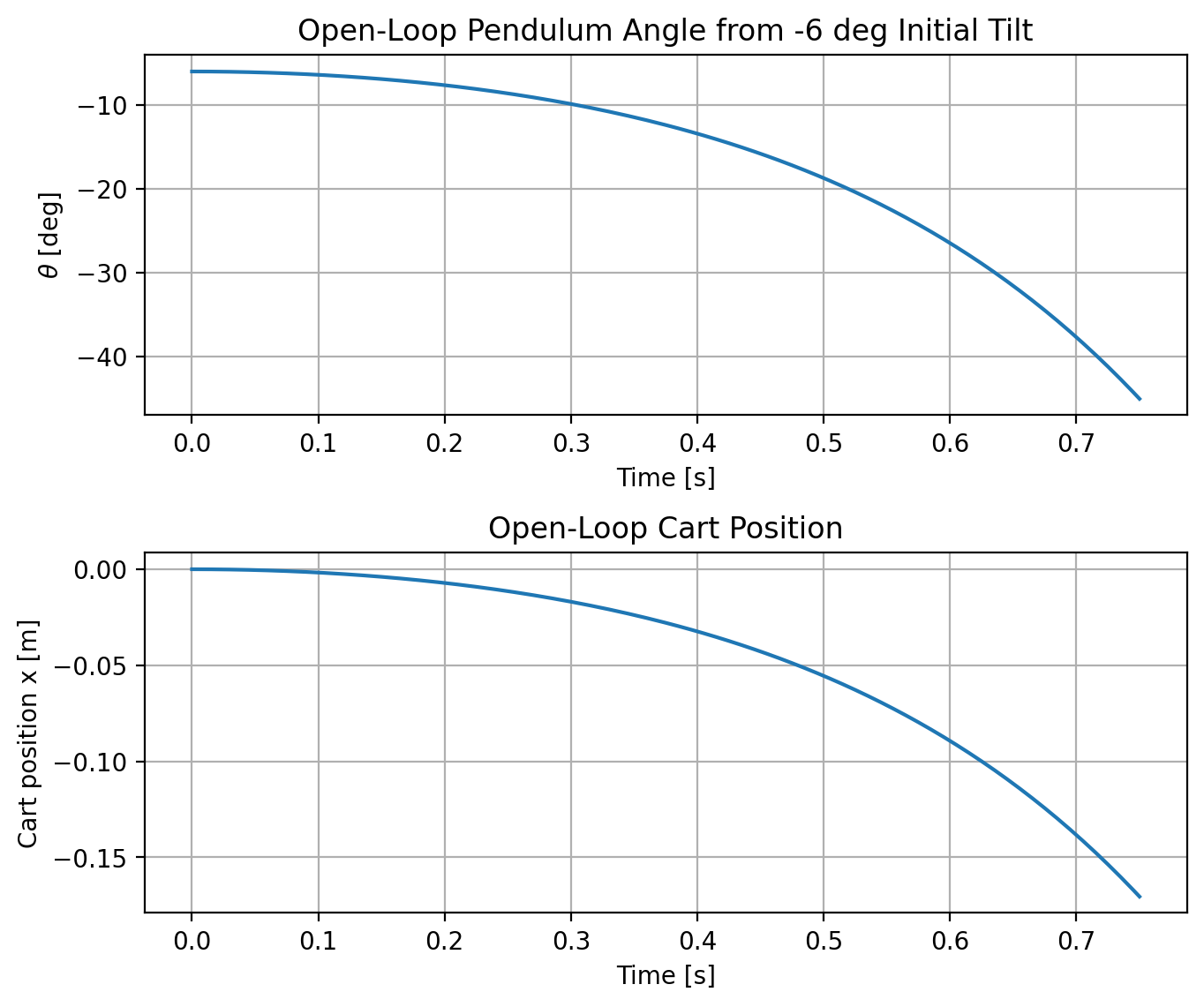
The positive real pole confirms the expected open-loop instability. The diagnostic trajectory is intentionally limited to the first 0.75 s because a large-angle trajectory from the linearized model would no longer be physically meaningful.

Short-horizon open-loop inverted pendulum instability — **Figure 1. Short-horizon open-loop instability.** Starting from a −6° initial tilt, the linear upright-equilibrium model diverges rapidly, consistent with its positive open-loop pole.

LQR design

The controller minimizes the continuous-time quadratic cost with Q = I. Two source-derived input penalties are compared: R = 0.1 for a more aggressive design and R = 50 for a lower-effort design. The cleaned runner solves the continuous-time algebraic Riccati equation through the Hamiltonian stable invariant subspace, so the project does not require Control System Toolbox.

R	Kx	Kθ	Kẋ	Kθ̇
0.1	−3.1623	72.6814	−6.6590	21.7140
50	−0.1414	43.6633	−0.8546	12.2307

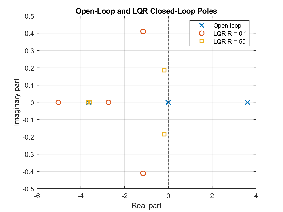
The Riccati residuals are approximately 1.47 × 10⁻¹³ for R = 0.1 and 2.13 × 10⁻⁸ for R = 50. Both feedback designs move all closed-loop poles into the left half-plane.

Open-loop and LQR closed-loop poles — **Figure 2. Open-loop and LQR closed-loop pole locations.** Both LQR designs stabilize the upright-equilibrium linear model, while the higher input penalty leaves a much slower dominant closed-loop pair.

Regulation from a −6° initial tilt

Closed-loop state responses for two LQR designs — **Figure 3. Closed-loop state responses.** The more aggressive R = 0.1 controller drives the states toward equilibrium faster and with substantially less cart travel.

Metric	R = 0.1	R = 50
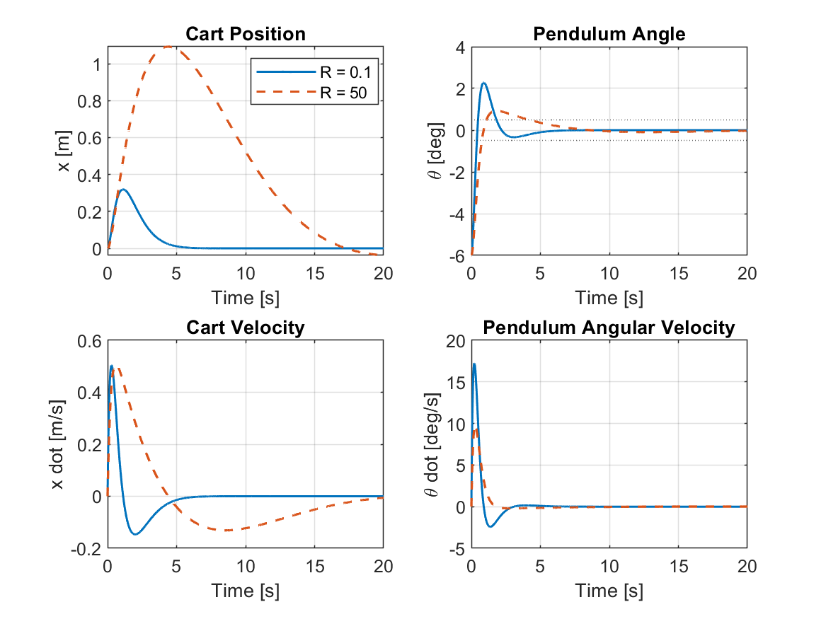
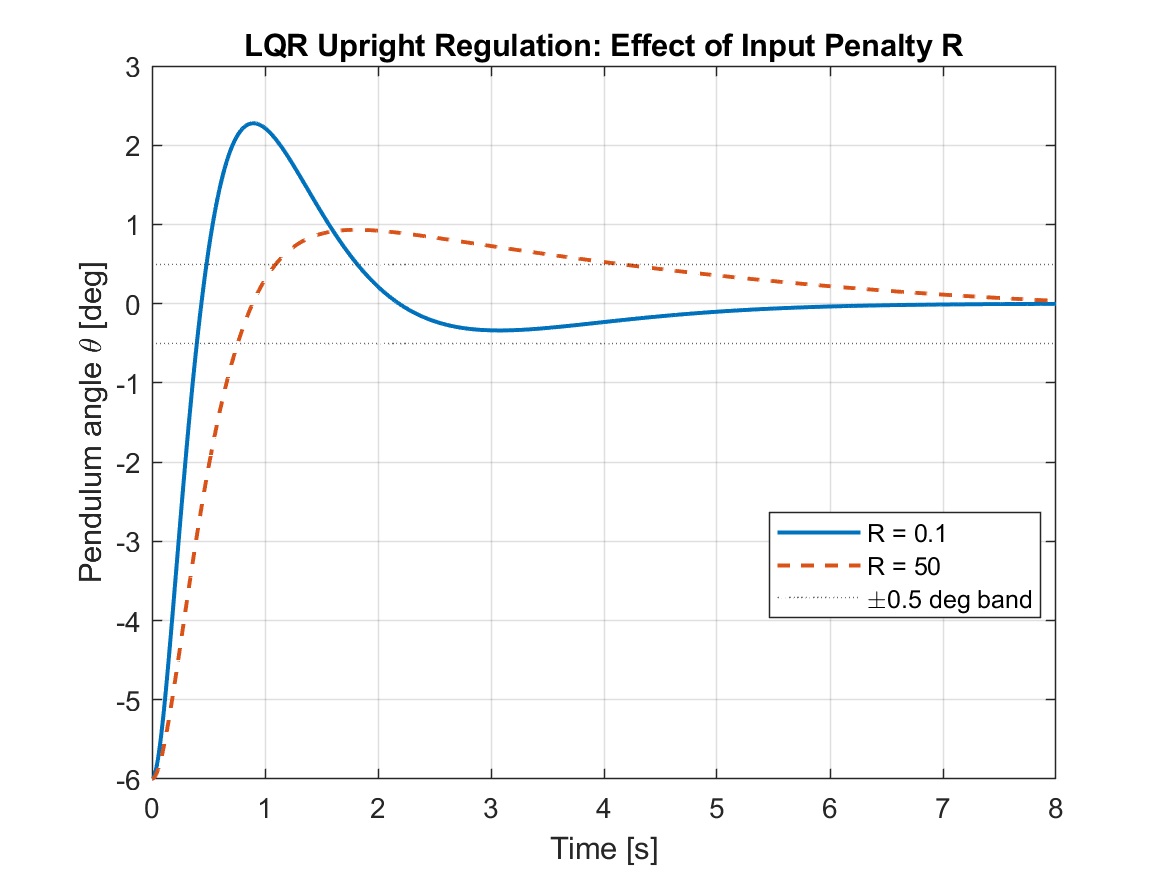
Angle settling time to ±0.5°	1.815 s	4.140 s
Peak cart excursion	0.319 m	1.092 m
Peak control force	7.611 N	4.572 N
Integral control effort, ∫u²dt	5.008 N²s	2.744 N²s

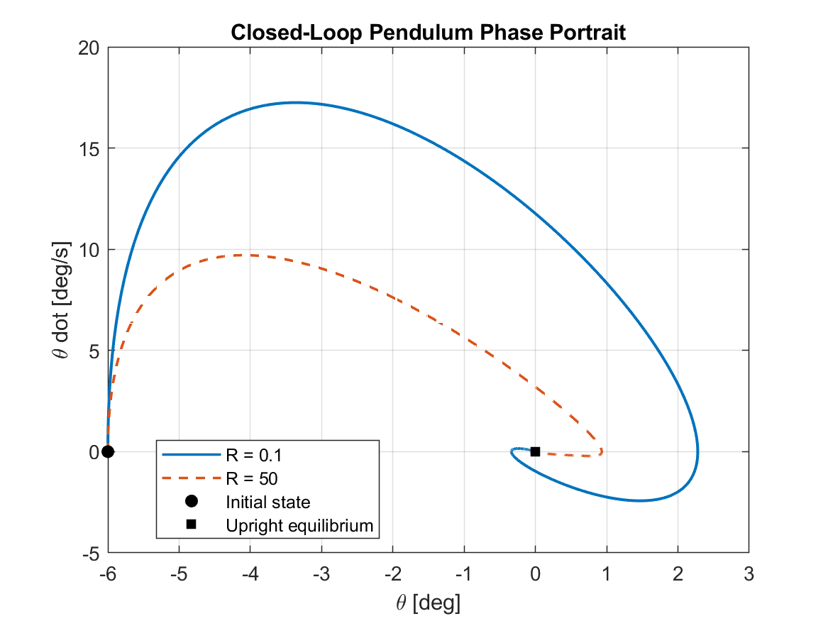
Reducing the input penalty gives faster regulation and smaller cart excursion, but requires higher peak and integrated control effort. Increasing R reduces effort but produces a slower, more weakly damped closed-loop response.

Pendulum angle regulation under two LQR input penalties — **Figure 4. Pendulum-angle regulation.** The R = 0.1 design enters and remains inside the ±0.5° band substantially earlier than the R = 50 design.

Control-effort tradeoff

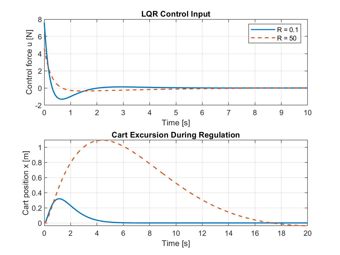
LQR control force and cart excursion — **Figure 5. Control force versus cart excursion.** The lower-effort controller reduces peak force, but the cart moves more than three times farther before the slow mode decays.

For R = 50, the slow closed-loop pair is approximately −0.1915 ± 0.1845j. The pendulum angle can therefore be close to zero while the cart state is still slowly returning toward equilibrium. The nonzero full-state norm at 20 s is a slow stable transient, not a loss of stability.

Phase-plane behavior

**Figure 6. Closed-loop pendulum phase portrait.** Both trajectories converge to the upright equilibrium, with the higher-effort design approaching it more rapidly.

Animation

Animated cart inverted-pendulum stabilization under LQR control — **Animated cart–pendulum regulation.**

Scope and limitations

The plant is a linearized upright-equilibrium model.
The main validation starts from −6° so the experiment remains close to the small-angle regime.
The archived separate 45° demo is not used as evidence for this linear model.
Full-state feedback is assumed; no state observer is used in the closed-loop study.
Actuator saturation, sensor noise, parameter uncertainty, and hardware experiments are not included.
The old Simulink animation model is not redistributed because its callback provenance is not fully attributable to this project.
The new MATLAB animation is visualization only; it does not add dynamics beyond the simulated state-space model.

Reproducibility

The repository is organized around one entry point:

run_inverted_pendulum_lqr_project

A complete run regenerates the state-space checks, LQR gains, poles, metrics, seven static figures, and animated GIF. The final published results were validated with MATLAB R2022b.